The basic premise of this activity is to be able to estimate the area of a figure with defined edges using Green’s theorem and Scilab. Green’s theorem generally relates a double integral over a certain region with a line integral around that region. The equation is given by:
Where the F’s are functions. By choosing appropriate functions we can reduce this equation such that we have an equation to determine the area of a closed region:
 Which in discretized form yields:
Using the final form of the equation, we can now determine the area of an image with the aid of scilab. We begin by generating black and white images of simple shapes using Scilab or paint. I used MS Paint for this part as I find it easier to draw these images than generate ones. It must be noted that the figure of interest must be in white while the background is in black. I picked a square and circle as my test subjects.
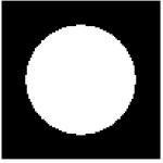
Images of the shapes I used to test Green’s theorem
For the square, it was found that:
area computed using green’s theorem= 9751.5 square pixels
actual area = 9801. square pixels
error = 0.5050505 %
The actual area was obtained by getting the number of pixels in one row of the figure and squaring it.^
For the circle, the values obtained were:
area computed using green’s theorem=84623.5 square pixels
actual area = 73541.542 square pixels
error = 15.068976 %
In this case the actual area was obtained by getting the number of pixels along the diameter and using the equation for the area of a circle which is A= Πr^2
It is noticeable that the discrepancy between the error values for the two shapes are quite big. This may be attributed to the fact that a real circle has a smooth curved edge which is what is assumed in the equation for the area of a circle. However, actual data, which was used for the computation of area using Green’s theorem, does not exactly resemble a perfectly smooth curved edge, instead it is approximated with small squares with finite value as can be clearly seen by magnifying the object. Thus the discrepancy between the error values lies in the difference between the assumptions and actual data for the two shapes.
Scilab code:
/part 1
//square
image= imread(‘D:\files\kaye\186\square.bmp’); //load image to scilab
[sqx , sqy] = follow(image); //folows contour of binary object
x=length(sqx);
//green’s theorem
for i = 1:x-1
sq(i)=sqx(i)*sqy(i+1)-sqx(i+1)*sqy(i);
end
area = sum(sq)/2
actual = (max(sqx)-min(sqx))^2 //actual area
error = ((actual-area )/actual)*100
//circle
circle = imread(‘D:\files\kaye\186\circle.bmp’);
[circx , circy] = follow(circle);
x=length(circx);
//green’s
for i = 1:x-1
circ(i)=circx(i)*circy(i+1)-circx(i+1)*circy(i);
end
area = sum(circ)/2
actual = (((max(circx)-min(circx))/2)^2)*%pi
error = (abs(actual-area )/actual)*100
The second part of this activity is applying the technique to real life. Particularly, the land area of a desired location will be computed using the same way as presented above. I chose the Ninoy Aquino International Airport Terminal 3 (NAIA 3) as my test subject for this part.
NAIA 3 is the most recent and biggest among the terminals of the said Airport. It’s building 182, 500 square meters and was build on a 63.5 hectares of land.

Ninoy Aquino international Airport terminal 3 bird's eye view

A rendering of NAIA terminal 3
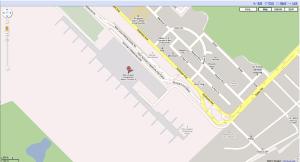
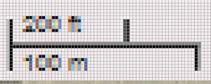
First I looked for NAIA terminal 3 in Google Maps to have a scaled image of its land area. Using the scale bar provided by Google maps, I was able to find how many square meters each square pixels represents by the same technique as in Activity 1.
The map was editted such that NAIA terminal 3 was left, it was then turned to a black and white image where the land area of the terminal was left white while the whole background was turned to black.
Using the same technique as above the following observations were made:
scaling factor = 2.972652 with an uncertainty of 0.000297
naia3_area = 533619.2 square meters
error =193.19736 %
There was a big discrepancy between the actual area of the terminal and the area I was able to compute. Some of the possible reasons for this error are:
- The method I used to separate the terminal from the rest of the image is not accurate at all, I might have included some area that I should not have or the other way around.
- The actual area I compared with my results is the area for the building only. I am not, however, aware of the actual boundaries of this ‘building’. I may have included parts of the terminal that are not really accounted for as part of that ‘building’.
- The uncertainty with the scaling factors I’ve used.
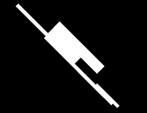
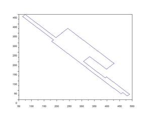
I think I should have used the total land area of 68.5 hectares or 685000 square meters because then my error would go down to 15.96548 %. I guess I’m really at lost with what is the actual area of the part I computed for although I think it does not really matter since I was able to do what I was supposed to. As a proof that I computed for the right area I plot the contour of the image I followed and got:
Which resembles the area of interest I was computing. From here I could say that I was doing the right thing except for comparing with the right values.
I give myself a grade of 9 for this activity. Although I have a huge error for the second part, I was able to apply the technique successfully for the other parts implying that I have learned what I have to learn.
I would like to thank Rob Entac for sharing some ideas on this activity and Jonathan Abat for tellingme how to check if I’m really following the right contour.
References:
[1] A2 – Area Estimation for Images with Defined Edges Manual prepared by Dr. Maricor Soriano, 2010
[2] http://en.wikipedia.org/wiki/Ninoy_Aquino_International_Airport
for the images:
[4] http://www.airport-technology.com/projects/ninoaquino/ninoaquino1.html
[5] http://mymanila-ph.blogspot.com/2008/07/manila-international-airport-t3.html


