Act 11. Playing Notes by Image Processing

Musical score sheet

For this activity we will be using our image processing skills to be able to play the musical score sheet presented using Scilab. Due to the lack of time, I was not able to successfully achieve my goal here. I will still however, present on how I supposed the problem should have been attacked. First I will convert the  score sheet into a binarized image since most of our knowledge deals with them. It would be helpful to divide the image into smaller segments that are easier to handle such as a single line. Correlation must then be implemented to determine the notes one segment at a time.

Sample binarized segment of the entire score sheet

Act 13. Color Image Segmentation

In activity 10 we have successfully specified our Region of Interest (ROI) by morphological operations and filtering out regions with certain area measurement. For this activity, we will again be dealing with specifying ROI, only this time we will be using the color of the ROI to do so.

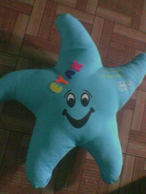
We begin by finding an image of an object with roughly monochromatic color. Figure 1 shows the image that I will be processing for this activity.

Figure 1. Image to be processed

A monochromatic region was then cropped. I chose 3 different regions – one from the bright side, one from the dark side, and one from the middle – for comparison. These regions are shown in figures 2-A, 2-B, and 2-C respectively.

Figure 2-A ROI 1

Figure 2- B ROI 2

Figure 2- C. ROI 3

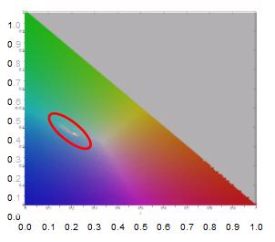
A 2D histogram of the ROIs were obtained for the non-parametric segmentation. It was also used to check if my code is working as it was supposed to. By comparing the histogram to the RG chromaticity diagram provided I can check if I’m getting the right histogram. A sample comparison can be seen in figure 3. For a clear comparison I used a colormap to plot the histogram of the ROI instead of the usual 2D plots. I then superimposed a semi-translucent chromaticity diagram in the colormap. The light pixels, encircled in the figure, indicate the points where the histogram has a high value. It can be clearly seen that these pixels coincide with the cyan-ish region of the given diagram which is the color of the ROI.

Figure 3. Histogram of sample ROI (colormap) superimposed with RG Chromaticity Diagram

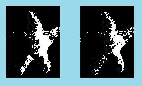
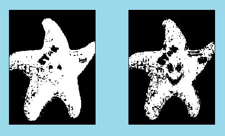
Image processed using Parametric (left) and Non-parametric (right) Segmentation using the ROI 1

Image processed using Parametric (left) and Non-parametric (right) Segmentation using ROI 2

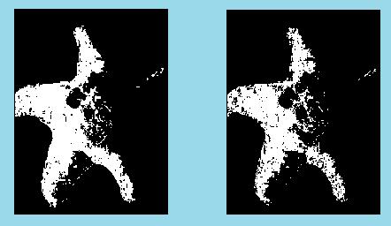
Image processed using Parametric (left) and Non-parametric (right) Segmentation using ROI 3

It can be noticed that when the ROI was cropped from the dark side the resulting image showed less of the bright side while the opposite happened when theROI was cropped from the bright side. Getting the ROI from the middle resulted to an image that is closest to the original image. This mean s that the middle area represents more of the colors in the desired image than the other two ROIs. Comparing the results of Parametric and Non-parametric segmentation we could see that the parametric one resulted to a cleaner image with more defined edges. The star shape which is the desired region was more clearly separated from the background using parametric segmentation. However, the non-parametric segmentation resulted to a more detailed image. Compared to that of the parametric, the details inside the ROI (which are not part of the ROI) are more defined in non-parametric segmentation. Overall, I would say that Parametric segmentation yields better results however, it depends largely on the desired application.

I would like to thank Jonats for sharing his insights

Grade: 9/10

— to be continued

Act 12. Color Image Processing

For the past activities we have always been working with either binary or grayscale images.  But wouldn’t it be a waste if we would just convert every image that we have to grayscale whenever we want to enhance it. In this activity, we will learn some image processing technique that will help enhance the quality of our images without giving up its color, well at least not all of it.

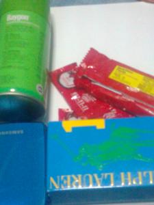
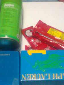
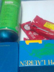
First we gather colorful images (with something white in the background) using different white balance options available with our camera. I used my Nokia 2700 camera phone for this so my images were not that highly resolve but they will do just fine. There are four white balance settings available in my phone – Auto, Daylight, Incandescent, and Fluorescent. The images obtained using these settings are shown in Figures 1-4.

Figure 1. White balance set to 'daylight'

Figure 2. White balance set to auto

Figure 3. White balance set to 'fluorescent'

Figure 4. White balance set to 'incandescent'

Among the four images the one captured using ‘Incandescent’ setting is chosen for enhancement since it looks a little too blue. This is probably in consideration for the yellow orange – ish color of the light coming from an incandescent bulb.

Figure 5. Image (left) processed using White Patch Algorithm (middle) and Gray World Algorithm (right)

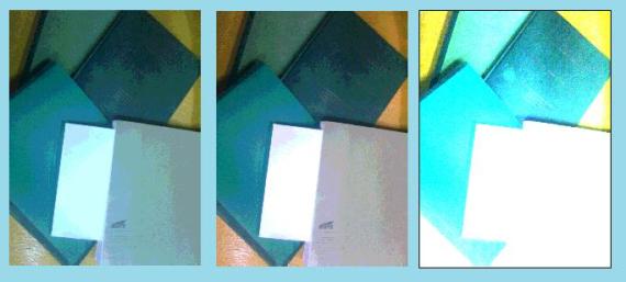
Figure 6. Image consisting of objects with the same hue (left) processed using White Patch Algorithm (middle) and Gray World Algorithm (right)

For the two examples, the white patch algorithm gave better results than the gray world algorithm.

I would like to thank Jonathan Abat for sharing his insights about this activity

Grade: 9/10

— to be continued

Act 10. Binary Operations

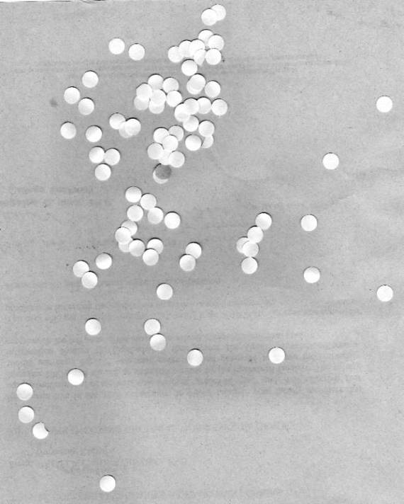
And so it is now time to apply what we have learned so far, or at least some of it. For this activity we will be using an image of scattered punched paper, shown in figure 1, which we will treat like cells. The objective is to be able to estimate the area of a single cell (one punched paper)

Figure 1. Image to be processed

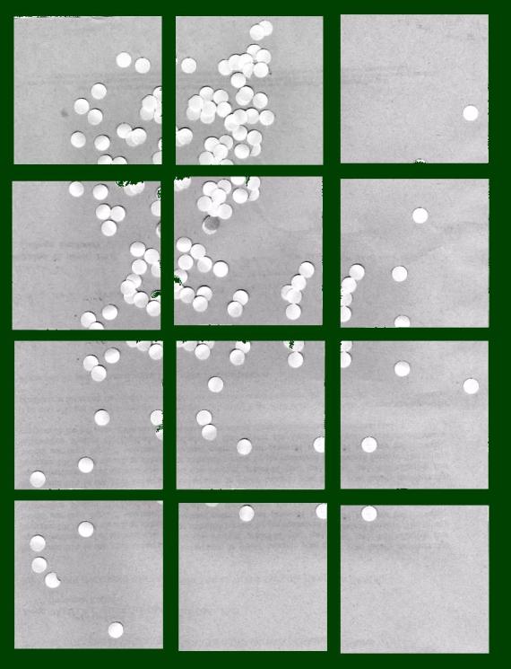
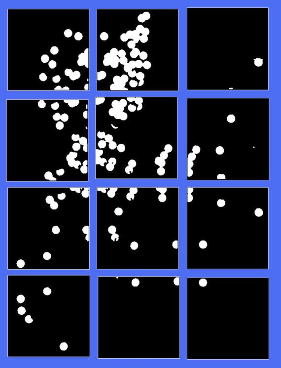
Part of the activity is to be able to design the program such that it will process one sub-image at a time in a loop. This could easily be done using for loop and naming each subimage properly (i.e.: name1.jpg, name2.jpg, name3.jpg, …). So we divide the image first into twelve 256X256 subimages as shown in figure 2.

Figure 2. Original image cropped into twelve 256x256 images

We then binarized the images and perform opening and closing operations to clean them up and separate as much cells from one another as possible. The results are shown in figure 3. (Review: to open means to erode then dilate an image while to close means to dilate then erode an image)

Binarized images after closing and opening

The command ‘bwlabel’ was used to label each blob on the image. By analyzing the histogram of the area of each blob, one will have an idea on the range of area measurements that are possibly single cell. Using this range, we can filter the region(s) of interest. By averaging the areas of these ROI’s we can have our best estimate for the area of a cell which was found to be 514 pixels. For reference, I cropped an image of a single cell and computed for its area which is 500 pixels. My approach obtained an error of 2.8%.

Reference cell

— to be continued

Act 9. Morphological Operation

Morphological operations

Images to be processed. (Solid square, Triangle, Hollow square, Cross / Plus sign)

//Strels
one= [1 1;1 1];
two= [1 1];
three= [1 ; 1];
four= [1 0 1 ; 0 1 0 ;1 0 1];
five = [0 1; 1 0];

Solid Square

Dilation

Erosion

Triangle

Dilation

Erosion

Hollow Square

Dilation

Erosion

Cross

Dilation

Erosion

Effect of 'skeleton' command on the images

Effect of 'thin' command on the images

— to be continued

Act 8. Enhancement in the Frequency Domain

From previous activities we have familiarized ourselves with Fourier Transform, giving us idea on what result would we get if we apply FT on certain patterns. In this activity we would use our knowledge of Fourier Transform to enhance certain images by removing visible repetitive patterns on them using filter masks.

A. Convolution theorem

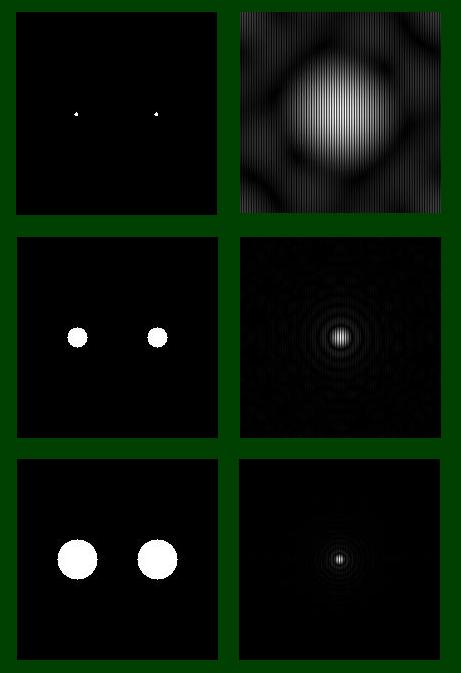
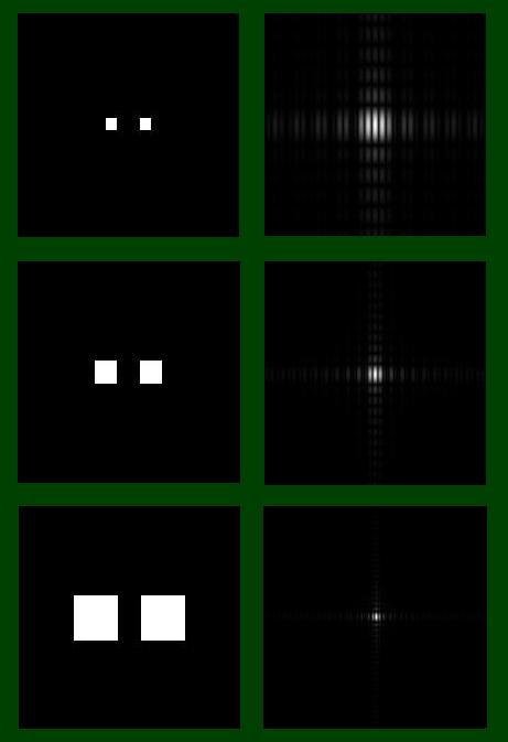
Before we do the actual filtering, we familiarize ourselves first with generating shapes and getting their FT’s using scilab, the convolution theorem, and working with dirac deltas.

Figure 1. Dots and their Fourier Transform

Figure 2. Circles of incresing radius (left) and their Fourier Transforms (right)

Figure 3. Squares of increasing widths (left) and their Fourier Transforms (right)

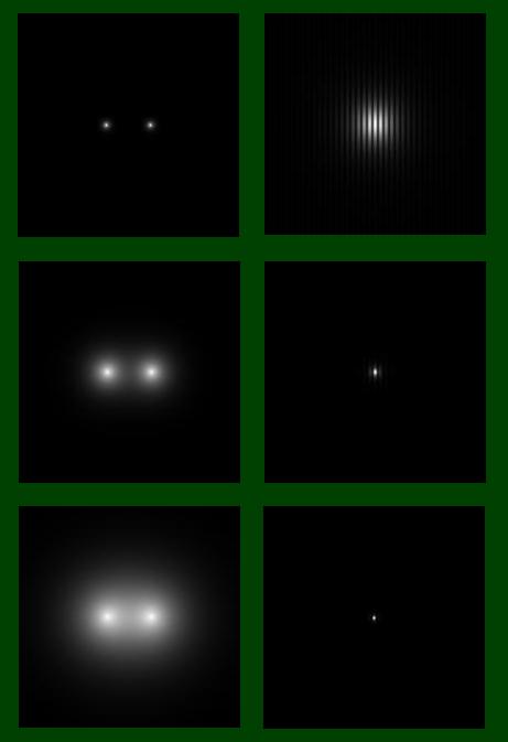
Figure 4. Gaussians of increasing variance (left) and their Fourier Transforms (right)

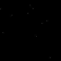
Dirac deltas in random locations

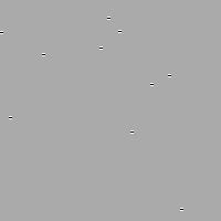
The above dirac deltas were convolved to two patterns:

a= [1 1 1 : -2 -2 -2 : 1 1 1 ];

b= [1 -2 1: 1 -2 1: 1 -2 1];

Convolution. Upper: dirac deltas convoloved with a. Lower: dirac deltas convolved with b

From the result of the convolution it is apparent that the patterns convolved with the dirac deltas were just repeated at the positions of the dirac deltas. This confirms the earlier statement that “The convolution of a dirac delta and a function f(t) results in a replicationof f(t) in the location of the dirac delta” from the manual.

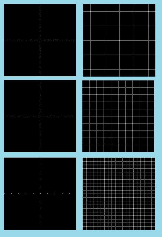
Arranged dirac deltas of increasing frequencies (top to bottom, left images) and their respective FT (right)

— to be continued…

Act 7. Properties of the 2D Fourier Transform

Fourier transform (2D): mathematical representation of an image as a series of two-dimensional sine waves.

-http://www.wadsworth.org/spider_doc/spider/docs/glossary.html

This activity deals with the properties of 2D Fourier Transform.

Familiarization with FT of Different 2D Patterns

For the first part of this activity, we were to familiarize ourseleves with Fourier Transform by applying it to several 2D patterns namely:

-square

-annulus

-square annulus

-2 slits

-2 dots

The resulting Fourier Transforms are shown below:

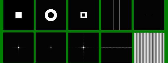
Figure 1. 2D patterns (top) and their fourier transform (bottom)

Anamorphic Property of the Fourier Transform

Here we investigate on how Fourier Transform varies with certain parameters in the patters. In particular, we want to know how the FT of a 2D sinusoid changes with varying frequency and rotation.

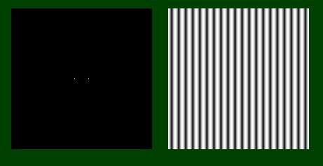
From the image below we could see that as we increase the frequency of the sinusoid the resulting FT of the pattern, 2 dots symmetric about the x axis, also increases in separation.

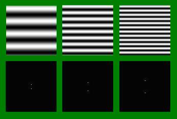
Figure 2.Top images are 2D sinusoids of increasing frequencies. Bottom images are their fourier transforms.

Rotating the sinusoids also produced a somewhat reverse effect to its FT, that is with respect to sinusoid that is parallel with the x-axis. In my example shown below, I rotated the sinusoids by 30 degrees and 45 degrees. Applying FT on the images resulted to 2 dots ‘rotated’ by approximately the same amount but in the other direction. (I know ‘rotated’ is not the proper term but I hope you get what I mean).

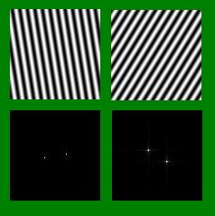
Figure 3. Rotated sinusoids (top) and their respective Fourier Transforms (bottom)

Finally, we look at how FT applies to combination of different patterns.  Below we see a series of combination of rotated sinusoids. Our base pattern is the first image shown which is a combination of 2 2D sinusoids, one parallel to the x-axias and another to the y-axis. We then add a third sinusoid rotated at different angles.

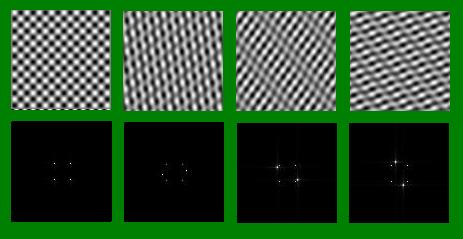
Figure 4. Combination of rotated sinusoids (top) and their fourier transforms (bottom)

Comparing their FT’s we could see that 4 dots seem to consistently appear in all four images while for the last three patterns two additional dots appeared which behaves comparable to that of the FT’s of the rotated sinusoids shown in Figure 3. The FT’s of the combined patterns seem to be a combination of the FT’s of their respective constituent patterns.

I would like to thank Mr. Entac and Mr. Abat for sharing their insights about this activity.

Grade: 9/10